Getting started with simChef

1 Overview

Welcome to simChef! Our goal is to empower data scientists to focus their attention toward scientific best practices by removing the administrative burdens of simulation design. Using simChef, practitioners can seamlessly and efficiently run simulation experiments using an intuitive tidy grammar. The core features of simChef include:

A tidyverse-inspired grammar of data-driven simulation experiments
A growing built-in library of composable building blocks for evaluation metrics and visualization utilities
Flexible and seamless integration with distributed computation, caching, checkpointing, and debugging tools
Automated generation of an R Markdown document to easily navigate, visualize, and interpret simulation results (see example here)

To highlight the ease of running simulation studies using simChef, we will begin by showcasing a basic example usage in Section 2. Then, in Section 3, we will provide additional details on how to create your own simulation experiment using simChef.

2 Example usage

Simulation Example: Suppose, for concreteness, that we would like to evaluate the prediction accuracy of two methods (linear regression and random forests) under a linear data-generating process across different signal-to-noise ratios.

At its core, simChef breaks down a simulation experiment into four components:

DGP(): the data-generating processes (DGPs) from which to generate data
Method(): the methods (or models) to fit on the data in the experiment
Evaluator(): the evaluation metrics used to evaluate the methods’ performance
Visualizer(): the visualization procedures used to visualize outputs from the method fits or evaluation results (can be tables, plots, or even R Markdown snippets to display)

Using these components, users can easily run a simulation experiment in six simple steps. Below, we summarize these steps and provide code for our running example.

Step 1. Define DGP, method, evaluation, and visualization functions of interest.

Recall that in our simulation example, we would like to study two methods (linear regression and random forests) under a linear DGP. We code this DGP (linear_dgp_fun) and methods (linear_reg_fun and rf_fun) via custom functions below.

#' Linear Data-Generating Process
#' 
#' @description Generate training and test data according to the classical
#'   linear regression model: y = X*beta + noise.
#' 
#' @param n_train Number of training samples.
#' @param n_test Number of training samples.
#' @param p Number of features.
#' @param beta Coefficient vector in linear regression function.
#' @param noise_sd Standard deviation of additive noise term.
linear_dgp_fun <- function(n_train, n_test, p, beta, noise_sd) {
  n <- n_train + n_test
  X <- matrix(rnorm(n * p), nrow = n, ncol = p)
  y <- X %*% beta + rnorm(n, sd = noise_sd)
  data_list <- list(
    X_train = X[1:n_train, , drop = FALSE],
    y_train = y[1:n_train],
    X_test = X[(n_train + 1):n, , drop = FALSE],
    y_test = y[(n_train + 1):n]
  )
  return(data_list)
}

#' Linear Regression Method
#' 
#' @param X_train Training data matrix.
#' @param y_train Training response vector.
#' @param X_test Test data matrix.
#' @param y_test Test response vector.
linear_reg_fun <- function(X_train, y_train, X_test, y_test) {
  train_df <- dplyr::bind_cols(data.frame(X_train), y = y_train)
  fit <- lm(y ~ ., data = train_df)
  predictions <- predict(fit, data.frame(X_test))
  return(list(predictions = predictions, y_test = y_test))
}

#' Random Forest Method
#' 
#' @param X_train Training data matrix.
#' @param y_train Training response vector.
#' @param X_test Test data matrix.
#' @param y_test Test response vector.
#' @param ... Additional arguments to pass to `ranger::ranger()`
rf_fun <- function(X_train, y_train, X_test, y_test, ...) {
  train_df <- dplyr::bind_cols(data.frame(X_train), y = y_train)
  fit <- ranger::ranger(y ~ ., data = train_df, ...)
  predictions <- predict(fit, data.frame(X_test))$predictions
  return(list(predictions = predictions, y_test = y_test))
}

We can similarly write custom functions to evaluate the prediction accuracy of these methods and to visualize results. However, simChef also provides a built-in library of helper functions for common evaluation and visualization needs. We leverage this library for convenience here. In particular, for prediction tasks, we will use the functions simChef::summarize_pred_err() and simChef::plot_pred_err() to evaluate and plot the prediction error between the observed and predicted responses, respectively. For details, see ? simChef::summarize_pred_err and ? simChef::plot_pred_err.

Note: Most of the user-written code is encapsulated by Step 1. From here, there is minimal coding on the user end as we turn to leverage the simChef grammar for experiments.

Step 2. Convert functions into `DGP()`, `Method()`, `Evaluator()`, and `Visualizer()` class objects.

Once we have specified the relevant DGP, method, evaluation, and visualization functions, the next step is to convert these functions into DGP(), Method(), Evaluator(), and Visualizer() class objects (R6) for simChef. To do so, we simply wrap the functions in create_dgp(), create_method(), create_evaluator(), or create_visualizer(), while specifying (a) an intelligible name for the object and (b) any input parameters to pass to the function. For example,

## DGPs
linear_dgp <- create_dgp(
  .dgp_fun = linear_dgp_fun, .name = "Linear DGP",
  # additional named parameters to pass to .dgp_fun()
  n_train = 200, n_test = 200, p = 2, beta = c(1, 0), noise_sd = 1
)

## Methods
linear_reg <- create_method(
  .method_fun = linear_reg_fun, .name = "Linear Regression"
  # additional named parameters to pass to .method_fun()
)
rf <- create_method(
  .method_fun = rf_fun, .name = "Random Forest", 
  # additional named parameters to pass to .method_fun()
  num.threads = 1
)

## Evaluators
pred_err <- create_evaluator(
  .eval_fun = summarize_pred_err, .name = 'Prediction Accuracy',
  # additional named parameters to pass to .eval_fun()
  truth_col = "y_test", estimate_col = "predictions"
) 

## Visualizers
pred_err_plot <- create_visualizer(
  .viz_fun = plot_pred_err, .name = 'Prediction Accuracy Plot',
  # additional named parameters to pass to .viz_fun()
  eval_name = 'Prediction Accuracy'
)

Step 3. Assemble recipe parts into a complete simulation experiment.

Thus far, we have created the many individual components (i.e., DGP(s), Method(s), Evaluator(s), and Visualizer(s)) for our simulation experiment. We next assemble or add these components together to create a complete simulation experiment recipe via:

experiment <- create_experiment(name = "Example Experiment") %>%
  add_dgp(linear_dgp) %>%
  add_method(linear_reg) %>%
  add_method(rf) %>%
  add_evaluator(pred_err) %>%
  add_visualizer(pred_err_plot)

We can also vary across one or more parameters in the DGP(s) and/or Method(s) by adding a vary_across component to the simulation experiment recipe. In the running simulation example, we would like to vary across the amount of noise (noise_sd) in the underlying DGP, which can be done as follows:

experiment <- experiment %>%
  add_vary_across(.dgp = "Linear DGP", noise_sd = c(0.1, 0.5, 1, 2))

Tip: To see a high-level summary of the simulation experiment recipe, it can be helpful to print the experiment.

print(experiment)
#> Experiment Name: Example Experiment 
#>    Saved results at: results/Example Experiment 
#>    DGPs: Linear DGP 
#>    Methods: Linear Regression, Random Forest 
#>    Evaluators: Prediction Accuracy 
#>    Visualizers: Prediction Accuracy Plot 
#>    Vary Across: 
#>       DGP: Linear DGP 
#>          noise_sd:  num [1:4] 0.1 0.5 1 2

Step 4. Document and describe the simulation experiment in text.

A crucial component when running veridical simulations is documentation. We highly encourage practitioners to document:

the purpose or objective of the simulation experiment,
what DGP(s), Method(s), Evaluator(s), and Visualizer(s) were used, and
why these DGP(s), Method(s), Evaluator(s), and Visualizer(s) were chosen.

This can and should be done before even running the simulation experiment. To facilitate this tedious but important process, we can easily initialize a documentation template to fill out using

init_docs(experiment)

Step 5. Run the experiment.

At this point, we have created and documented the simulation experiment recipe, but we have not generated any results from the experiment. That is, we have only given the simulation experiment instructions on what to do. To run the experiment, say over 100 replicates, we can do so via

results <- run_experiment(experiment, n_reps = 100, save = TRUE)
#> Fitting Example Experiment...
#> Saving fit results...
#> Fit results saved | time taken: 0.105875 seconds
#> 100 reps completed (totals: 100/100) | time taken: 3.391054 minutes
#> ==============================
#> Evaluating Example Experiment...
#> Evaluation completed | time taken: 0.099427 minutes
#> Saving eval results...
#> Eval results saved | time taken: 0.055685 seconds
#> ==============================
#> Visualizing Example Experiment...
#> Visualization completed | time taken: 0.001210 minutes
#> Saving viz results...
#> Viz results saved | time taken: 0.478525 seconds
#> ==============================

Step 6. Visualize results via an automated R Markdown report.

Finally, to visualize and report all results from the simulation experiment, we can render the documentation. This will generate a single html document, including the code, documentation (from Step 4), and simulation results.

render_docs(experiment)

The rendered document corresponding to this simulation example can be found here, and voila! Simulation example complete!

In the next section, we will provide additional details necessary for you to create your own simulation experiment.

3 Writing your own simulation experiment

When it comes to writing your own simulation experiment using simChef, the main task is writing the necessary DGP, method, evaluation, and visualization functions for the experiment (i.e,. step 1 above). Once these functions are appropriately written/specified, simChef takes care of the rest, with steps 2-6 requiring very little effort from the user.

Thus, focusing on step 1, it is helpful to understand the inputs and outputs that are necessary for writing each user-defined function. To do so, let us walk through what happens when we run a simChef Experiment and highlight the necessary inputs and outputs to these functions as we go.

Overivew of running an experiment

At the highest level, running an experiment (via run_experiment()) consists of three main steps (see Figure 3.1):

Fit each Method on each DGP (and for each of the varying parameter configurations specified in vary_across) via fit_experiment().
Evaluate the experiment according to each Evaluator via evaluate_experiment().
Visualize the experiment according to each Visualizer via visualize_experiment().

run_experiment() is simply a wrapper around these three functions: fit_experiment(), evaluate_experiment(), and visualize_experiment().

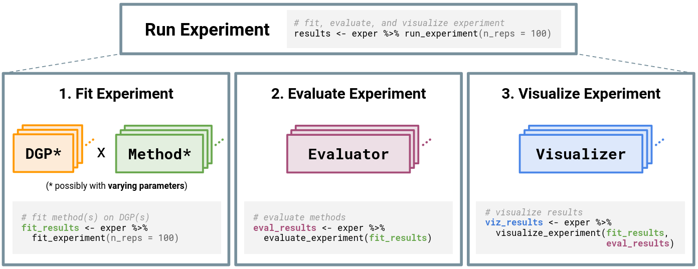
Overview of running a simChef Experiment. The Experiment class handles relationships among the four classes: DGP(), Method(), Evaluator(), and Visualizer(). Experiments may have multiple DGPs and Methods, which are combined across the Cartesian product of their varying parameters (represented by *). Once computed, each Evaluator and Visualizer takes in the fitted simulation replicates, while Visualizer additionally receives evaluation summaries.

In what follows, we will discuss fitting, evaluating, and visualizing the experiment, each in turn.

Fitting an experiment

When fitting an experiment, each Method is fit on each DGP (for each specified vary_across parameter configuration). As such, the outputs of the user-defined DGP functions should match input arguments to the user-defined Method functions. More specifically,

DGP inputs:
- Any number of named parameters (e.g., dgp_param1, dgp_param2, …)
DGP outputs:
- A list of named elements to be passed onto the method(s) (e.g., dgp_out1, dgp_out2, …)
Method inputs:
- Named parameters matching all names in the list returned by the DGP function (e.g., dgp_out1, dgp_out2, …)
- Any number of additional named parameters (e.g., method_param1, method_param2, …)
Method outputs:
- A list of named elements (e.g., method_out1, method_out2, …) [Note: this output list should contain all information necessary to evaluate and visualize the method’s performance]

Finally, fit_experiment() returns the fitted results across all experimental replicates in a tibble. This tibble contains:

Identifier columns
- .rep: replicate ID
- .dgp_name: name of DGP
- .method_name: name of Method
- vary_across parameter columns (if applicable): value of the specified vary_across parameter
A column corresponding to each named component in the list returned by the Method (e.g., method_out1, method_out2, …)

We summarize these inputs and outputs in Figure 3.2.

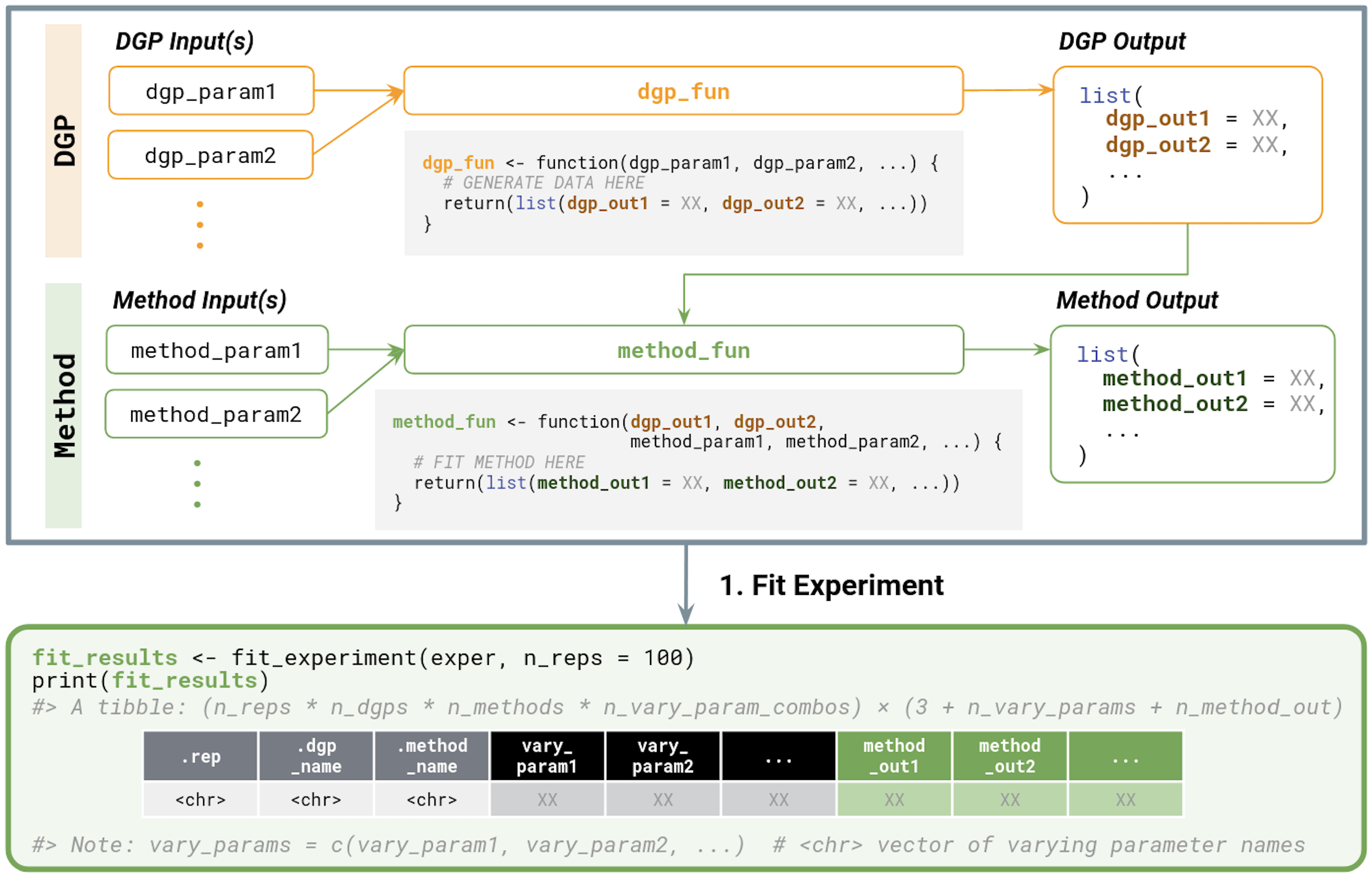
Overview of fitting a simChef Experiment. Inputs and outputs for user-defined functions are also provided.

Evaluating an experiment

Next, when evaluating an experiment, the output of fit_experiment() (i.e., fit_results from Figure 3.2) as well as a character vector of the vary_across parameter names (i.e., vary_params) are automatically passed to each Evaluator function. Typically, an Evaluator takes the fit_results tibble in as input, evaluates some metric(s) on each row or group of rows (e.g., summarizing across replicates), and returns the resulting tibble or data.frame. We summarize the relevant inputs and outputs below and in Figure 3.3.

Evaluator inputs:
- fit_results (optional): output of fit_experiment()
- vary_params (optional): character vector of parameter names that are varied across in the experiment
- Any number of additional named parameters (e.g., eval_param1, eval_param2, …)
Evaluator outputs:
- Typically a tibble or data.frame

The output of evaluate_experiment is a named list of evaluation result tibbles, one component for each Evaluator in the experiment. Here, the list names correspond to the names given to each Evaluator in create_evaluator(.name = ...), and the list elements are exactly the return value from the Evaluator function.

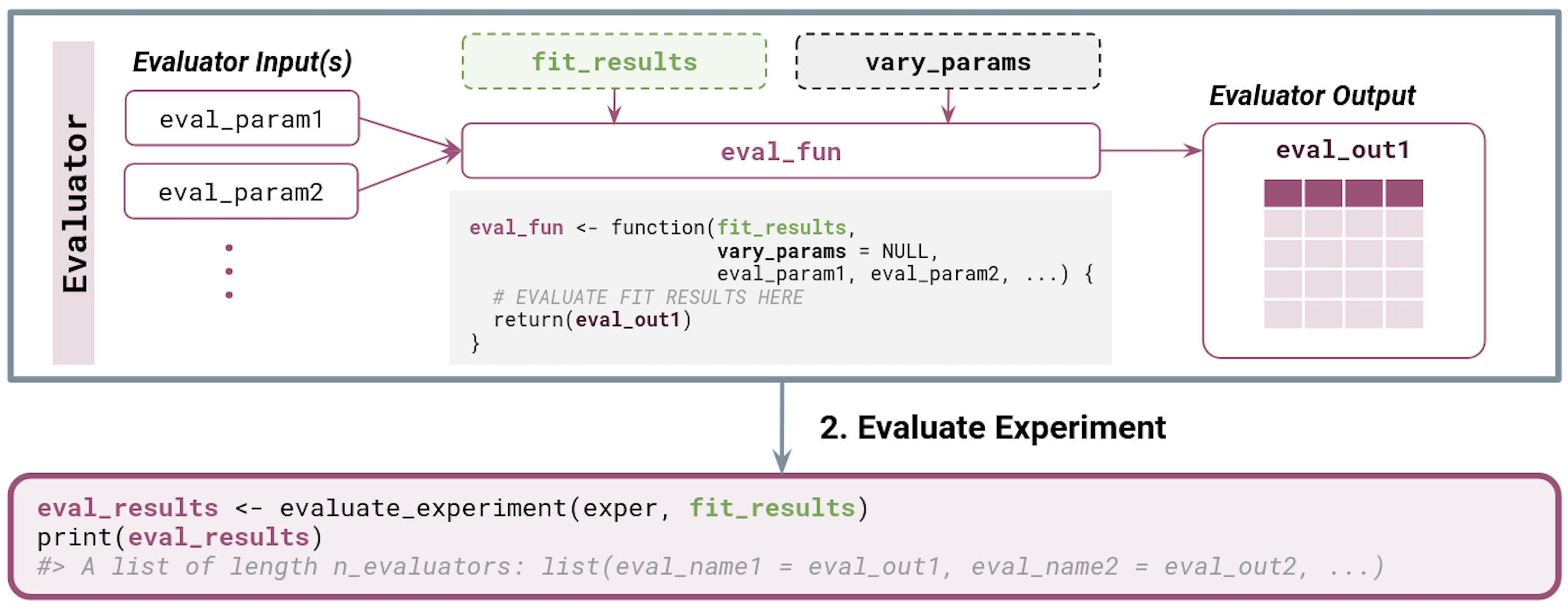
Overview of evaluating a simChef Experiment. Inputs and outputs for user-defined functions are also provided. Dotted boxes denote optional input arguments.

Visualizing an experiment

In the last step, when visualizing an experiment, the output of fit_experiment() and evaluate_experiment (fit_results and eval_results, respectively) as well as vary_params are automatically passed to each Visualizer function. Typically, a Visualizer takes in the fit_results and/or eval_results and constructs a plot to visualize the performance of various methods (perhaps, across the varying parameter specified by vary_params). We summarize the relevant inputs and outputs below and in Figure 3.4.

Visualizer inputs:
- fit_results (optional): output of fit_experiment()
- eval_results (optional): output of evaluate_experiment()
- vary_params (optional): character vector of parameter names that are varied across in the experiment
- Any number of additional named parameters (e.g., viz_param1, viz_param2, …)
Visualizer outputs:
- Typically a plot (e.g., a ggplot or plotly object)

The output of visualize_experiment is a named list of visualizations or plots, one component for each Visualizer in the experiment. Here, the list names correspond to the names given to each Visualizer in create_visualizer(.name = ...), and the list elements are exactly the return value from the Visualizer function.

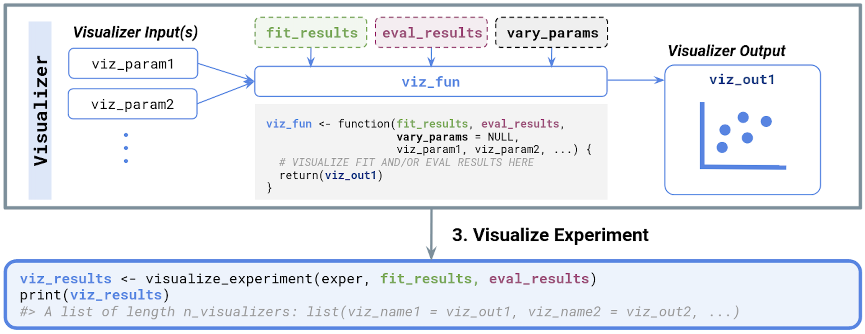
Overview of visualizing a simChef Experiment. Inputs and outputs for user-defined functions are also provided. Dotted boxes denote optional input arguments.

Putting it all together

As alluded to previously, once the DGP, Method, Evaluator, and Visualizer functions have been defined, the hard work has been done. For convenience, we provide below a template that can be used to run an experiment, assuming that dgp_fun, method_fun, evaluator_fun, and visualizer_fun have been appropriately defined.

## Step 2: Create DGP, Method, Evaluator, Visualizer class objects
dgp <- create_dgp(
  .dgp_fun = dgp_fun, .name = "DGP Name",
  # additional named parameters to pass to .dgp_fun()
  dgp_param1 = XXX, dgp_param2 = XXX, ...
)
method <- create_method(
  .method_fun = method_fun, .name = "Method Name",
  # additional named parameters to pass to .method_fun()
  method_param1 = XXX, method_param2 = XXX, ...
)
evaluator <- create_evaluator(
  .eval_fun = evaluator_fun, .name = "Evaluator Name",
  # additional named parameters to pass to .eval_fun()
  eval_param1 = XXX, eval_param2 = XXX, ...
)
visualizer <- create_visualizer(
  .viz_fun = visualizer_fun, .name = "Visualizer Name",
  # additional named parameters to pass to .viz_fun()
  viz_param1 = XXX, viz_param2 = XXX, ...
)

## Step 3: Assemble experiment recipe
experiment <- create_experiment(name = "Experiment Name") %>%
  add_dgp(dgp) %>%
  add_method(method) %>%
  add_evaluator(evaluator) %>%
  add_visualizer(visualizer) %>%
  # optionally vary across DGP parameter(s)
  add_vary_across(.dgp = "DGP Name", dgp_param1 = list(XXX, XXX, ...)) %>%
  # optionally vary across Method parameter(s)
  add_vary_across(.method = "Method Name", method_param1 = list(XXX, XXX, ...))

## Step 4: Document experiment recipe
init_docs(experiment)

## Step 5: Run experiment
results <- run_experiment(experiment, n_reps = 100, save = TRUE)

## Step 6: Render experiment documentation and results
render_docs(experiment)

4 Additional Resources

For more information on simChef and additional features, check out:

simChef culinary school (tutorial slides)
Computing experimental replicates in parallel (vignette)
Setting up your simulation study (vignette)
Cheat sheet: Inputs/outputs for user-defined functions (vignette)
simChef: A comprehensive guide (vignette) for information on caching, checkpointing, error debugging, common simulation experiment templates, and more
Case Study #1 using simChef to develop a new flexible approach for predictive biomarker discovery with rendered documentation here

Additional simChef examples/case studies and built-in library functions are still to come. Stay tuned!